Data structures and algorithms, referred to as DSA, is an advanced topic in computer science.
At macro level, data and correspondingly requirement for data analysis is growing exponentially, different use cases get created with this in every domain. It is thus a requirement to store and operate on data efficiently. Storage has become cheap hence efficiency/speed is more important now.
Efficiency in context of speed is one of the most needed property of a computer program. Managing storage and operations is a major factor on which efficiency of a program depends.
There are multiple ways to increase performance.
At micro level, a program instructs CPU to perform operations which take time.
All these operations happen at very large scale even in simple programs, e.g. basic data analysis. Therefore designing how the data is structured (data structure) and operated upon (algorithms) allows reducing these operations to improve performance.
Computer scientists are involved in rigorous study of the topic, including math involved, to come up with new data structures and algorithms. There are 2 main challenges
As a user, the problem is to match the right data structure if it exists with the use case.
As an advanced user or developer there might be a need to implement needed data structures.
Some languages like Python provide implementation of basic data structures as default while others like C leave it to the users to implement.
In Python, sequence types like list and tuple, mapping types like set and dictionary are all end result of this field of study, and are implemented and provided by default.
The choice of data structure decides available algorithms for different operations implemented for a data structure.
Choosing the data structure depends on use case
This section of the course aims to present and introduce some of the core results which are used currently, along with context and intuition behind the developments in the field. This should help
The study of data structures and algorithms can be summarized as below.
|
Interface |
Data structure & Algorithms |
|---|---|
|
Interface is a specification of structure of data and operations that should be supported |
Data structure is a implementation to store data with specified structure Algorithms for a given data structure are the implementation of operations |
|
Interface is a specification |
Data structure with Algorithms is an implementation |
|
Interface is the problem definition |
Data structure with algorithms is a solution |
|
There could be multiple data structures for the same interface, performance will be different |
A data structure might solve multiple interfaces, performance will be different |
There are 2 major costs involved while using a data structure
Measuring time and memory usage depends on 2 factors
Typically time is more critical as memory is considered cheap in the context of present day computer hardware.
Computational model refers to abstracting hardware performance in general terms to study the behavior of different operations to be performed. Typically word RAM model is used in theoretical studies. In practice it may differ.
Implication of assumptions in word RAM model are that all elementary operations take constant amount of time
RAM => Random access memory
Time complexity of an algorithm can be measured in different ways based on different contexts.
Measuring time directly has following disadvantages
It is more useful to measure time in terms of operations performed and then see how they grow with size of data. Using this approach isolates dependency on machine.
Using best case time for deciding time complexity might give false results as an algorithm might be fast on small data size but perform slow on large data size.
Using average time will give more information, but for that the probability distribution is needed to decide which data sizes will be used more frequently. It is very difficult to get an accurate distribution hence this option is not feasible.
Worst case time is used as it ensures bound on performance and reduces noise in comparing performance of different algorithms.
Time complexity is measured for worst case performance, using asymptotic notation for number of operations performed depending on data size, usually represented with \(n\).
Asymptotic notation is used to get an idea of asymptotic growth ignoring scaling factors and constants. More formally, asymptotic notation represents a set of functions.
Asymptotic growth simply means how the growth of a function behaves when the underlying variable grows too large. For example, if the the performance of an algorithm for a data structure takes the form \(T(n) = 3n^2\), what is the growth in value of \(T(n)\) as \(n \to \infty\), where \(T(n)\) is the time the algorithm takes and \(n\) is the size of data structure.
Below are the set of asymptotic notations.
|
Name |
Notation |
Description |
|---|---|---|
|
Asymptotically Equal |
\(f \sim g\) | |
|
Big O |
\(f \in O(g)\) |
upper bound |
|
Omega |
\(f \in \Omega(g)\) |
lower bound |
|
Theta |
\(f \in \Theta(g)\) |
both upper and lower bound |
|
Small O |
\(f \in o(g)\) |
strictly larger |
|
Little Omega |
\(f \in \omega(g)\) |
strictly smaller |
Theta and Big O are mostly used in measuring complexity.
The notation is some times used as \(f(n) = O(g(n))\) but it is more accurate to use \(f(n) \in O(g(n))\) as \(O(g(n))\) denotes a collection of functions.
Definition 21.1 (O Notation) A non-negative function \(f(n)\) is in \(O(g(n))\) if and only if there exist constants \(c, n_0 \in \mathbb{R}\) such that \(f(n) \le c \cdot g(n) \quad \forall \ n > n_0\).
Definition 21.2 (Omega Notation) A non-negative function \(f(n)\) is in \(\Omega(g(n))\) if and only if there exist constants \(c, n_0 \in \mathbb{R}\) such that \(f(n) \ge c \cdot g(n) \quad \forall \ n > n_0\).
Definition 21.3 (Theta Notation) A non-negative function \(f(n)\) is in \(\Theta(g(n))\) if and only if \(f(n) \in (O(g(n)) \cap \Omega(g(n)))\).
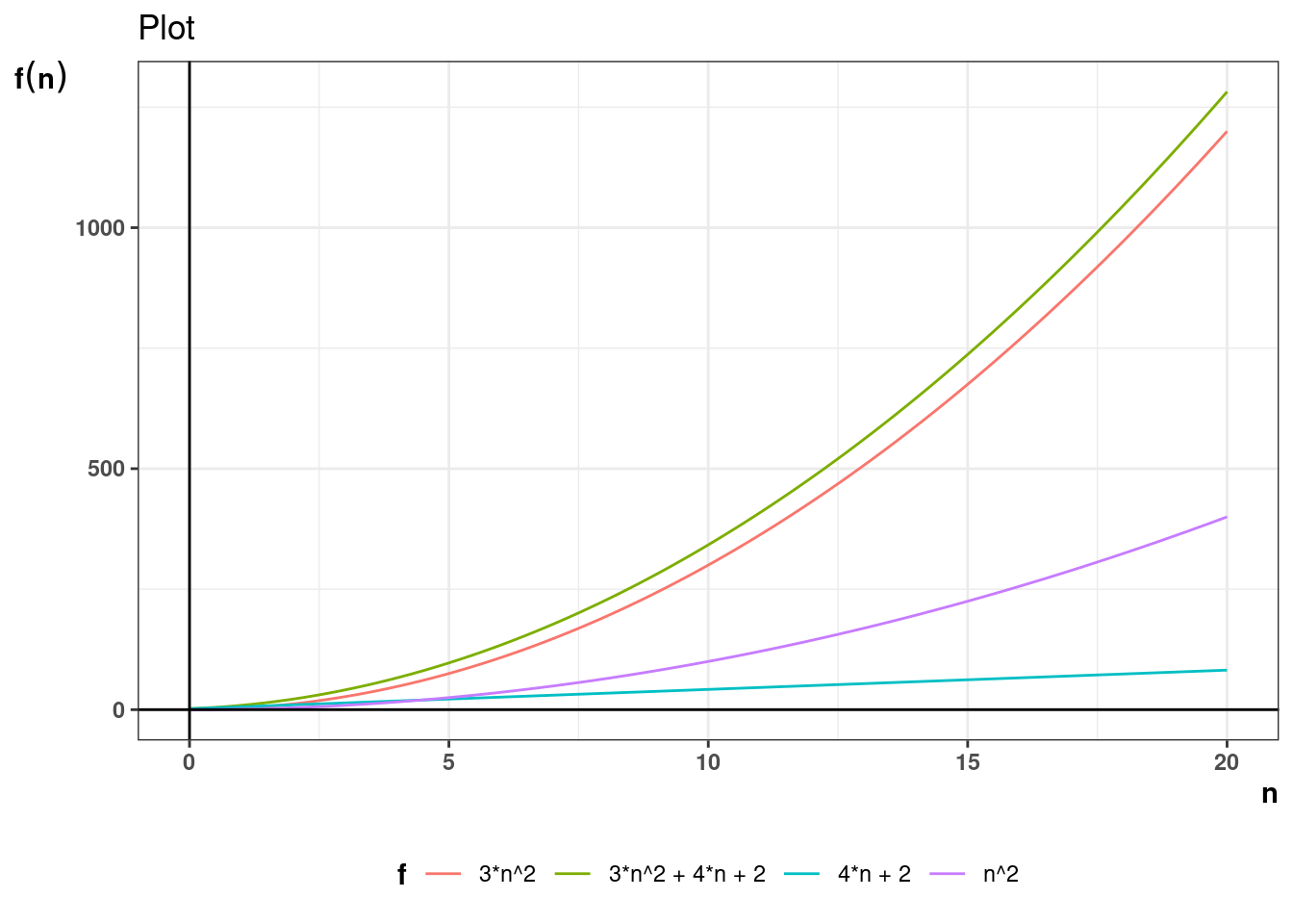
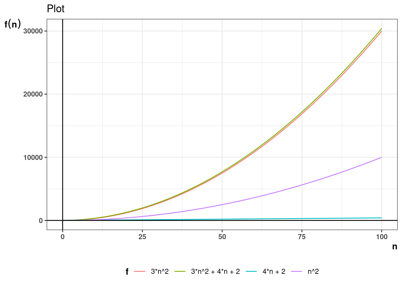
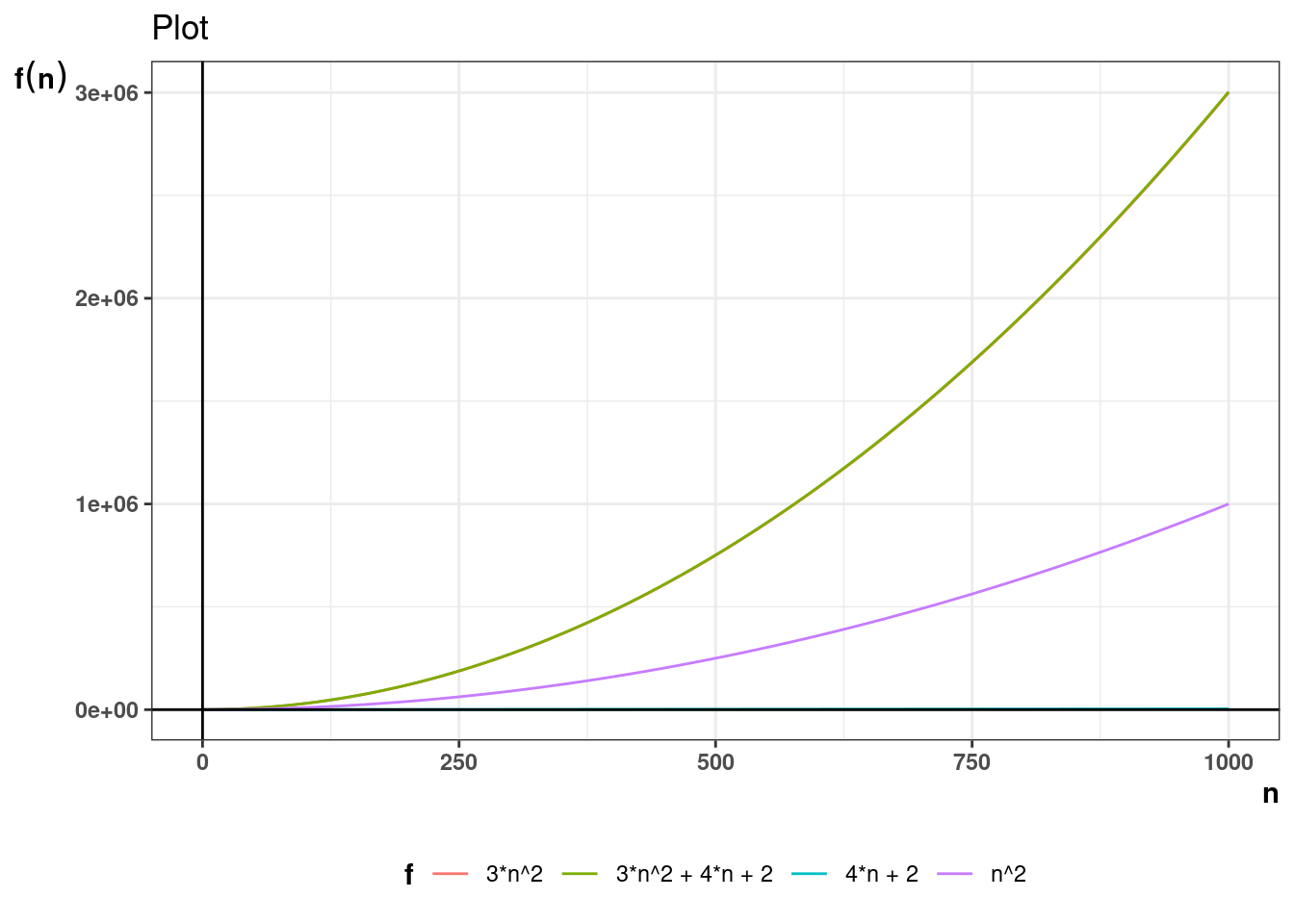
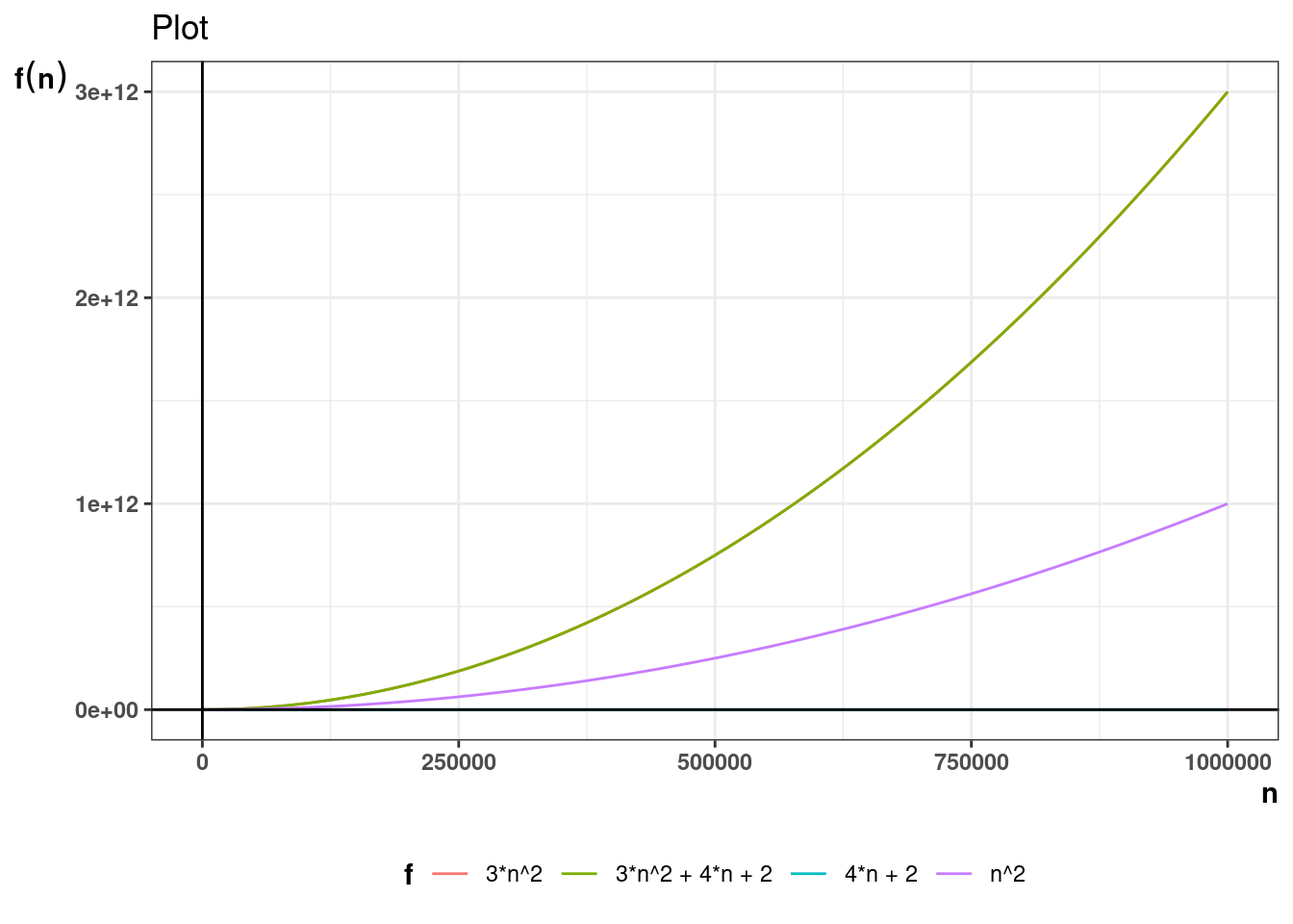
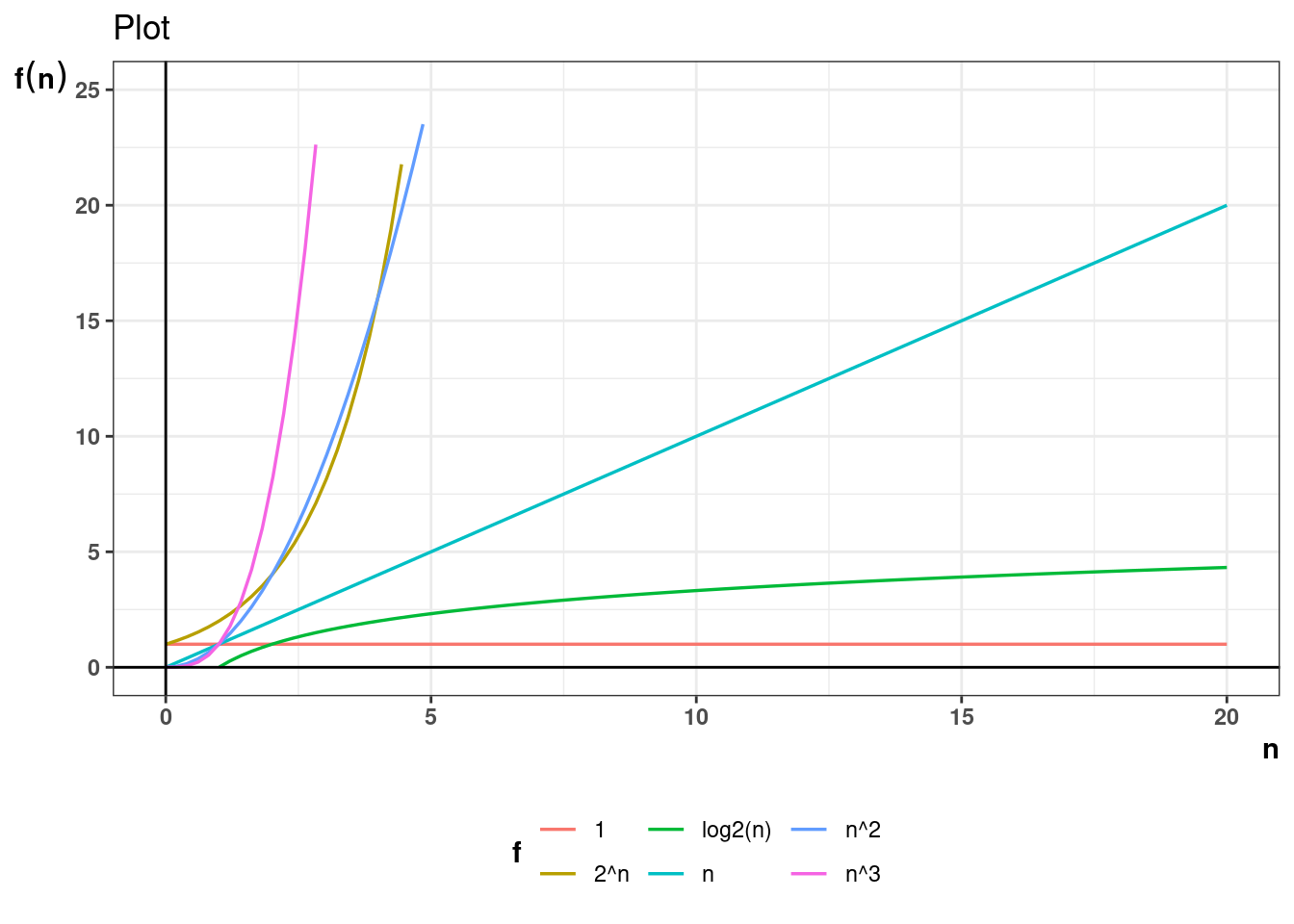
For example, if it is concluded that number of operations in an algorithm is given by the function \(T(n) = 3n^2 + 4n+ 2\) then \(T(n) \in \Theta(n^2)\). Theta notation allows for stating complexity in simpler terms ignoring scaling and constant factors.
Below plots show how the \(n^2\) term dominates as n grows larger.
In terms of efficiency of algorithms it is often desired to keep the complexity low. Below are the common functions which complexity takes in increasing order. Anything below linear is considered good.
| Constant | Logarithmic | Linear | Quadratic | Polynomial | Exponential |
|---|---|---|---|---|---|
| \(\Theta(1)\) | \(\Theta(log(n))\) | \(\Theta(n)\) | \(\Theta(n^2)\) | \(\Theta(n^c)\) | \(2^{\Theta(n^c)}\) |
Interface provides the abstract or theoretical requirements of storing and operating on certain type of data. For example, tuple, list or dictionary is used depending on the use case. Abstraction and generalization of use cases is interface. Tuple, list and dictionary are the implementation or data structures.
Interfaces are also referred to as
There are 2 main types of interfaces.
Operations on major interfaces can be categorized into 3 basic types
Below tables summarize the common operation specifications for sequence and mapping interfaces.
|
Category |
Method |
Description |
|---|---|---|
|
Container |
build(I) |
build a sequence from items in iterable |
|
len(x) |
return number of items |
|
|
Static |
iter_seq(x) |
return stored items one at a time in sequence order |
|
get_at(i) |
return the item at index i |
|
|
set_at(i, x) |
replace the item at index i with x |
|
|
Dynamic |
insert_at(i, x) |
add x as i^th item |
|
delete_at(i) |
remove and return i^th item |
|
|
insert_first(x) |
add x as the first item |
|
|
delete_first() |
remove and return 1^st item |
|
|
insert_last(x) |
add x as the last item |
|
|
delete_last() |
remove and return last item |
|
Category |
Method |
Description |
|---|---|---|
|
Container |
build(I) |
build a sequence from items in iterable |
|
len(x) |
return number of items |
|
|
Static |
find(k) |
return stored item with key k |
|
Dynamic |
insert(x) |
add x to set with key x.key, replace if key exists |
|
delete(k) |
remove and return the item with key k |
|
|
Order |
iter_order() |
return the stored items one by one in key order |
|
find_min() |
return the item with smallest key |
|
|
find_max() |
return the item with largest key |
|
|
find_next(k) |
return the item with key larger than k |
|
|
find_prev(k) |
return the item with key smaller than k |
Data structures are the actual implementations of interfaces. There is no single data structure that solves all operations required in an interface efficiently. Different data structures solve a subset of operations efficiently.
Below are some basic categories of data structures with examples.
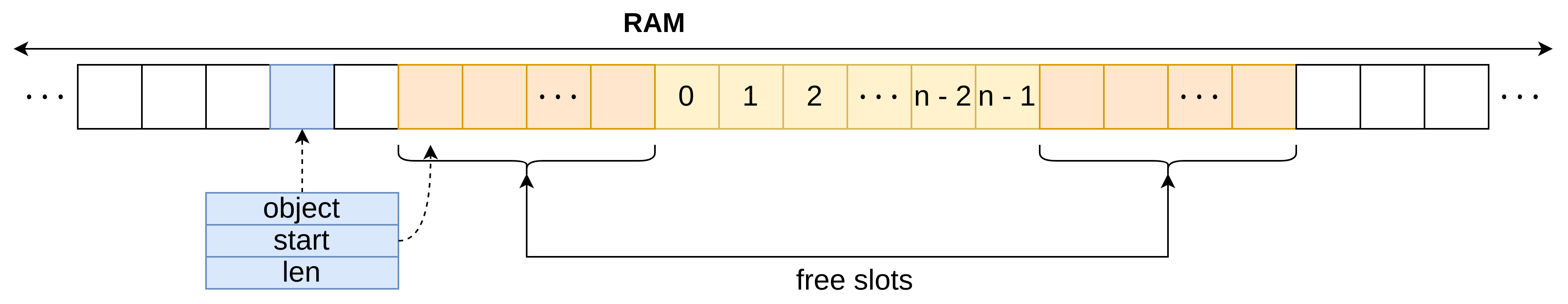
Random access memory (RAM) of computer hardware is like a giant continuous slots of memory addresses.
A static array finds and stores data in contiguous slots of equal size, depending on the size of data elements. The order is extrinsic, i.e. the items are stored in the order provided.
The static array object then needs to contain only the start memory address and length of the array.
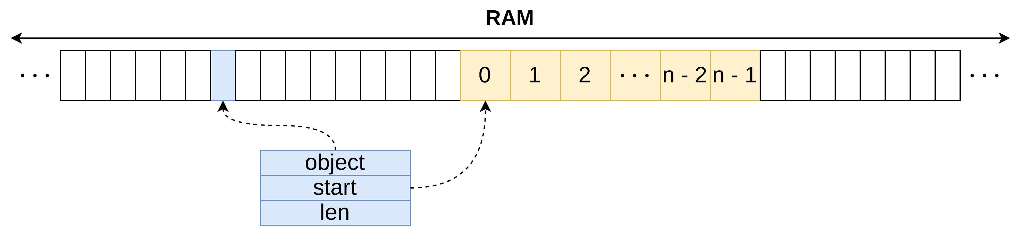
Python tuples are approximately static array, one main difference is tuples are immutable, i.e. modification operations are not supported, a new object is created on modification.
Below are tables for performance of static array for sequence and map operations. Static arrays are efficient for sequences with static operations only.
For dynamic operations, in the worst case new contiguous slot of free memory has to be looked and container has to be build, therefore it is \(O(n)\) operations.
| Data Structure | build(X) | get_at(i) set_at(i) | insert_first(x) delete_first() | insert_last(x) delete_last() | insert_at(i, x) delete_at(i) |
|---|---|---|---|---|---|
| array | n | 1 | n | n | n |
| Note: | |||||
| \(\cdot_{(a)}\) implies amortized, \(\cdot_{(e)}\) implies expected, h is height of the tree |
| Data Structure | build(X) | find(k) | insert(k) delete(k) | find_min() find_max() | find_prev(k) find_next(k) |
|---|---|---|---|---|---|
| array | n | n | n | n | n |
| Note: | |||||
| \(\cdot_{(a)}\) implies amortized, \(\cdot_{(e)}\) implies expected, h is height of the tree |
| Data Structure | build(X) | get_at(i) set_at(i) | insert_first(x) delete_first() | insert_last(x) delete_last() | insert_at(i, x) delete_at(i) |
|---|---|---|---|---|---|
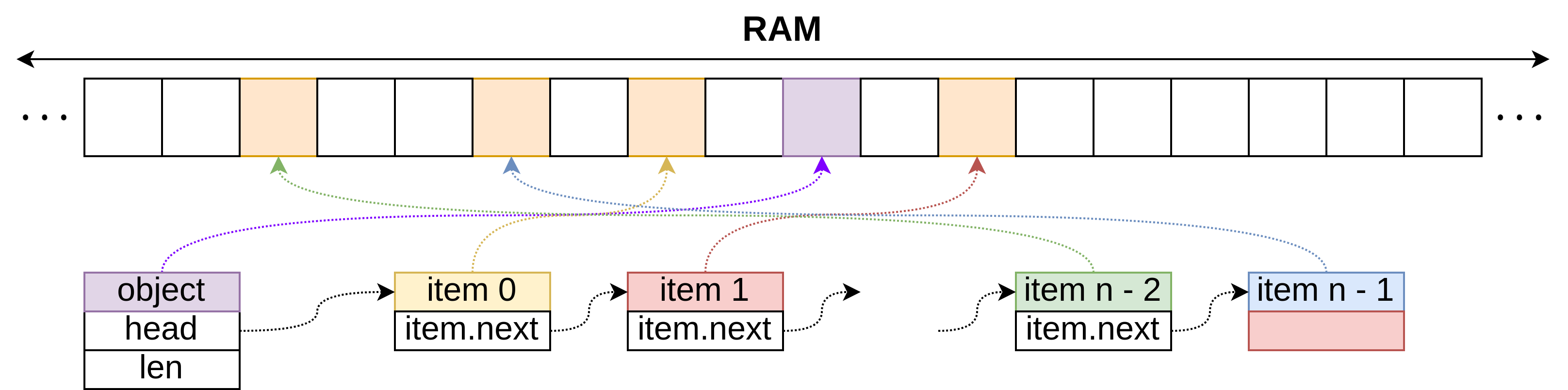
| linked list | n | n | 1 | n | n |
| Note: | |||||
| \(\cdot_{(a)}\) implies amortized, \(\cdot_{(e)}\) implies expected, h is height of the tree |
| Data Structure | build(X) | get_at(i) set_at(i) | insert_first(x) delete_first() | insert_last(x) delete_last() | insert_at(i, x) delete_at(i) |
|---|---|---|---|---|---|
| linked list | n | n | 1 | n | n |
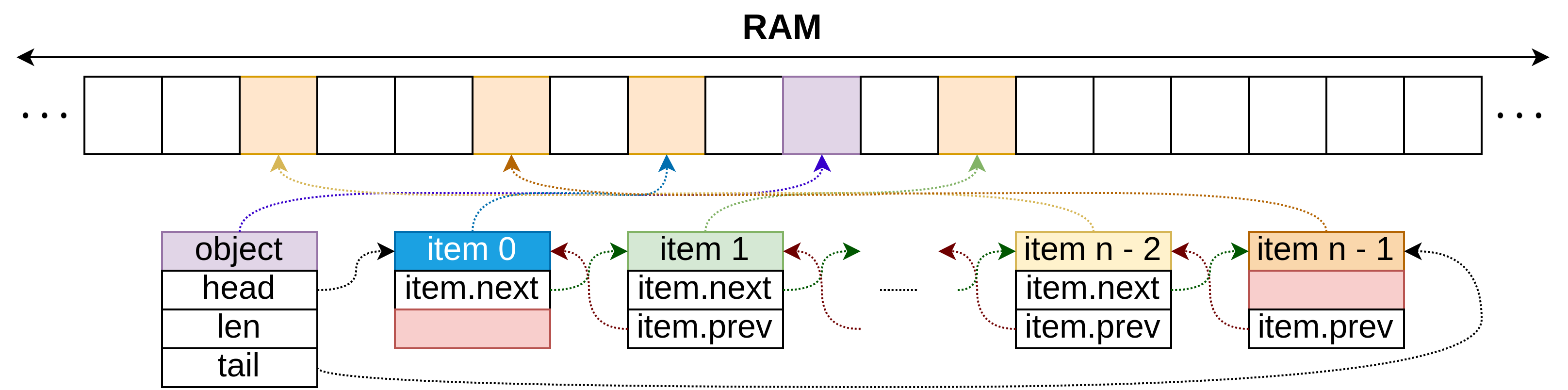
| doubly linked list w/ tail | n | n | 1 | 1 | n |
| Note: | |||||
| \(\cdot_{(a)}\) implies amortized, \(\cdot_{(e)}\) implies expected, h is height of the tree |
| Data Structure | build(X) | get_at(i) set_at(i) | insert_first(x) delete_first() | insert_last(x) delete_last() | insert_at(i, x) delete_at(i) |
|---|---|---|---|---|---|
| dynamic array | n | 1 | \(1_{(a)}\) | \(1_{(a)}\) | n |
| Note: | |||||
| \(\cdot_{(a)}\) implies amortized, \(\cdot_{(e)}\) implies expected, h is height of the tree |
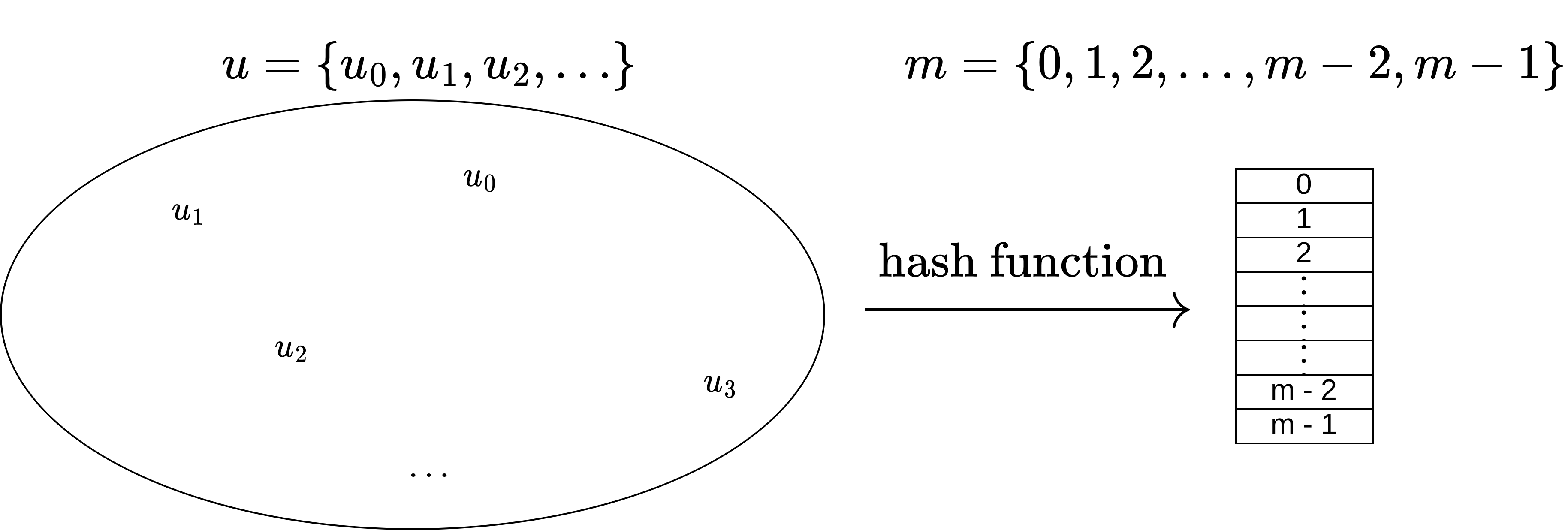
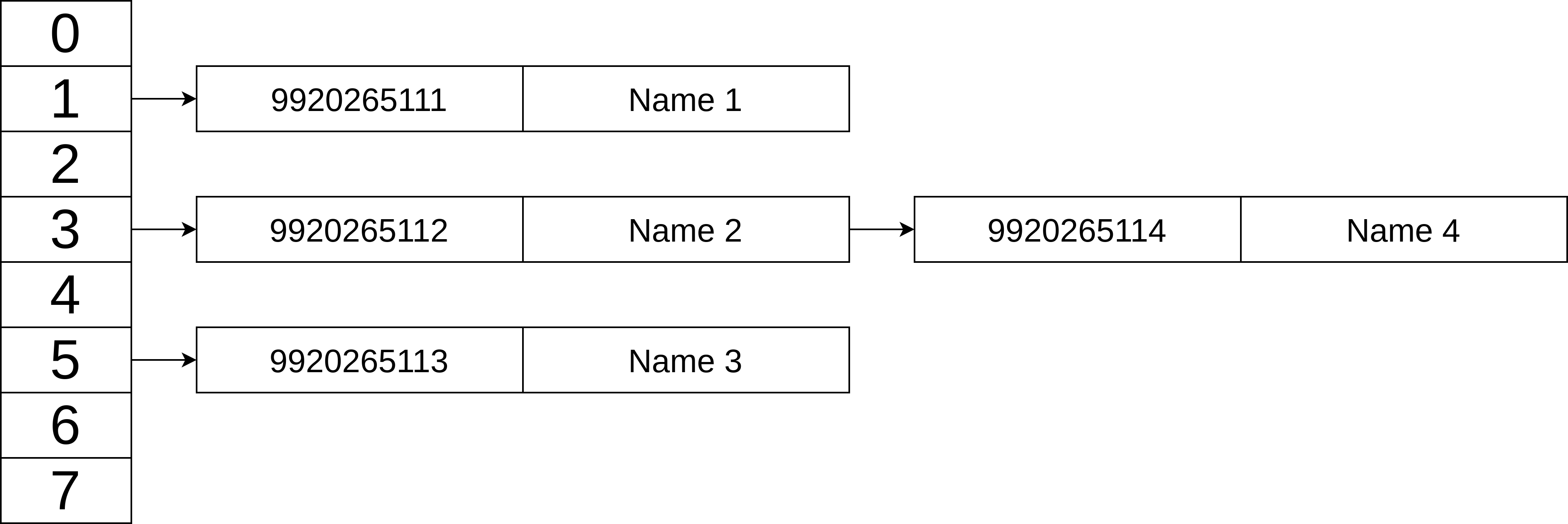
Hash tables are used to implement set interface: sets and dictionaries.
Taking example of a phone book where the requirements are
dict and set| Data Structure | build(X) | get_at(i) set_at(i) | insert_first(x) delete_first() | insert_last(x) delete_last() | insert_at(i, x) delete_at(i) |
|---|---|---|---|---|---|
| array | n | 1 | n | n | n |
| linked list | n | n | 1 | n | n |
| doubly linked list w/ tail | n | n | 1 | 1 | n |
| dynamic array | n | 1 | \(1_{(a)}\) | \(1_{(a)}\) | n |
| binary tree | n | h | h | h | h |
| avl tree | n | log n | log n | log n | log n |
| Note: | |||||
| \(\cdot_{(a)}\) implies amortized, \(\cdot_{(e)}\) implies expected, h is height of the tree |
| Data Structure | build(X) | find(k) | insert(k) delete(k) | find_min() find_max() | find_prev(k) find_next(k) |
|---|---|---|---|---|---|
| array | n | n | n | n | n |
| sorted array | n log n | log n (binary search) | n | 1 | log n |
| direct access array | u | 1 | 1 | u | u |
| hash tables | \(n_{(e)}\) | \(1_{(e)}\) | \(1_{(e)(a)}\) | n | n |
| binary tree | n log n | h | h | h | h |
| avl tree | n log n | log n | log n | log n | log n |
| Note: | |||||
| \(\cdot_{(a)}\) implies amortized, \(\cdot_{(e)}\) implies expected, h is height of the tree |
Algorithm is a procedure to solve a problem.
Study of algorithms involves study of finding correct and efficient procedures to solve problems.
Some classical algorithms are listed below along with their efficiency.
|
Application |
Name |
Performance |
Comments |
|---|---|---|---|
|
Search |
Linear search |
\(O(n)\) |
|
|
Binary search |
\(O(Log_2 \ n)\) |
|
|
|
Sort |
Insertion Sort |
\(O(n^2)\) |
|
|
Selection Sort |
\(O(n^2)\) |
|
|
|
Merge Sort |
\(O(n Log_2 \ n)\) |
|
An algorithm is a solution to implementing operations like search and sort for a data structure.
An operation for a implementation of a data structure can use any of the compatible algorithms, but not all will be efficient. For example, for sorting an array merge sort is much quicker than most algorithms.
The algorithms provided here should also serve as mini projects to research and implement the algorithm. This should be a good practice to apply combining basic building blocks in previous sections.